Active vs passive transformations in field theories

There’s a distinction between an active transformation and a passive one. In an active transformation, the actual value of a field at a given point in space or spacetime will change in general — you actually transform the field into a different field. In a passive transformation, you are not actually transforming any fields, you are merely changing the coordinate system you use to label points in your space, and if the field is described by a function of the coordinates, then that function changes so that you have a new function of the new coordinates that describes the same physical field as the old function of the old coordinates. I’ll argue that this difference affects how we think about what theories are allowed, so it’s important imo!

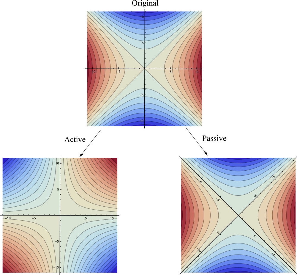
Fig. 1: Contour plots of temperature $T$ field (color), with active and passive rotations applied. We have the original temperature function $T(\mathbf x)$. After an active transformation, we have a new field described by $\widetilde{T}(\mathbf x) \equiv T(\mathbf R \mathbf x)$ where $\mathbf R$ is a rotation matrix that rotates a vector $45^\circ$ clockwise. Doing a passive transformation instead, we have the same physical field, but we have to describe it using a new function of the new coordinates $\mathbf r$: $\grave{T}(\mathbf r) \equiv T(\mathbf{R} \mathbf{r})$. In this case the two functions $\widetilde{T}(\cdot)$ and $\grave{T}(\cdot)$ are identical, which shows how easy it is to get confused!

As a concrete example, fig. 1 shows both types of transformation applied in the case of the temperature (scalar field) whose value is represented by color. Hopefully you agree that the two cases are different! If you place your hot friend at the location that has coordinates $(3,0)$ in the first picture, then after a passive transformation your friend will be exactly as hot as they were before because all you’ve done is call their location by a different name, whereas if the temperature field undergoes an active transformation, your friend may not be so hot anymore because the temperature at their location has actually changed! The two transformations lead to two different physical situations, because active transformations are transformations of physical fields, whereas passive transformations are merely relabellings of points, and point labels are completely arbitrary and unphysical.

This often comes up in the context of Lorentz transformations in relativistic field theories (quantum or classical). People often seem to gloss or omit the active-vs-passive distinction though, e.g. the wikipedia page on Lorentz Invariance ¹, the popular books by Peskin+Schroeder ², Srednicki ³, Zee ⁴, Ryder ⁵, and Kleinert ⁶, and the lecture notes by Gripaios ⁷. Tong’s excellent lecture notes ⁸ are better than most on this point, but still slip up in a few parts. Let’s discuss the sort of example that courses/books often have, first in an active way, then in a passive way…

Consider showing that the Klein-Gordon equation⁹ $$\partial_\mu \phi \, \eta^{\mu \nu} \, \partial_\nu \phi + k \phi = 0 \label{eq:kg}\tag{1}$$ is ‘Lorentz invariant’, where $\phi$ is a scalar field, $k$ is a constant, and $\eta$ is the metric tensor of Minkowski spacetime. Here, $\partial_\mu \equiv \partial / \partial x^\mu$ where $x^\mu$ is some coordinate system. What I think we mean by Lorentz invariance here is that if we have some field $\phi$ that solves the KG equation, then if we perform an active Lorentz transformation on $\phi$ to produce a new field $\tilde{\phi}$, then $\tilde{\phi}$ will also be a solution. Now, an active Lorentz transformation of the old field $\phi(x^a)$ produces a new field described by $\tilde{\phi}(x^a) \equiv \phi(\Lambda^a_{~b} x^b)$, where $\Lambda^a_{~b}$ is a constant Lorentz transformation matrix, analogously to fig. 1. Using chain rule, $$\partial_\mu \tilde{\phi}(x^a) = \partial_\mu \phi(\Lambda^a_{~b} x^b) = \Lambda^\nu_{~\mu} \bar{\partial}_\nu \phi(\Lambda^a_{~b} x^b) \label{eq:chain}\tag{2}$$ where $\bar{\partial}$ is a new operator that just differentiates a function with respect to its input arguments (‘slots’), rather than with respect to $x^\mu$. Eq. \ref{eq:chain} is just like in single-variable calculus where if you have $h(x) \equiv f(g(x))$ then $h’(x) = g’(x)f’(g(x))$, where the function $f’$ is the derivative of $f$ with respect to its argument. So we have $$\partial_\mu \tilde{\phi}(x^a) \, \eta^{\mu \nu} \, \partial_\nu \tilde{\phi}(x^a) + k \phi(x^a) = \Lambda^\rho_{~\mu} \bar{\partial}_\rho \phi(\Lambda^a_{~b} x^b) \eta^{\mu \nu} \Lambda^\sigma_{~\nu} \bar{\partial}_\sigma \phi(\Lambda^a_{~b} x^b) + k \phi(\Lambda^a_{~b} x^b).$$ Now we use the definitional property of the Lorentz transformation matrices $\Lambda^\rho_{~\mu} \eta^{\mu \nu} \Lambda^\sigma_{~\nu} = \eta^{\rho \sigma}$ to get $$\partial_\mu \tilde{\phi}(x^a) \, \eta^{\mu \nu} \, \partial_\nu \tilde{\phi}(x^a) + k \phi(x^a) = \bar{\partial}_\rho \phi(\Lambda^a_{~b} x^b) \eta^{\rho \sigma} \bar{\partial}_\sigma \phi(\Lambda^a_{~b} x^b) + k \phi(\Lambda^a_{~b} x^b). \label{eq:nearly}\tag{3}$$ Finally, we note that because $\phi(x^a)$ satisfies the KG eq. (\ref{eq:kg}) in which $\partial_\mu \equiv \partial / \partial x^\mu$, we actually have $\bar\partial_\mu \phi \, \eta^{\mu \nu} \, \bar\partial_\nu \phi + k \phi = 0$, no matter what value you feed into the left-hand side as a function argument! Thus the right-hand side of eq. \ref{eq:nearly} is zero and we have shown that $\tilde\phi$ is a solution of the KG equation: $$\partial_\mu \tilde{\phi}(x^a) \, \eta^{\mu \nu} \, \partial_\nu \tilde{\phi}(x^a) + k \phi(x^a) = 0 . \label{eq:kg2}\tag{4}$$

Now, lots of lecturers showing results like the above will write down strange things like “$x^a \rightarrow x’^a = \Lambda^a_{~b} x^b$”, which looks like a change of coordinates rather than anything active. The accompanying text is also often vague and passive-sounding. The problem with this imo is that the KG eq. (\ref{eq:kg}) is manifestly invariant under coordinate/passive transformations, because it is fully tensorial, written with correct upstairs and downstairs indices and whatnot! ANY genuine tensorial scalar is automatically invariant under ALL coordinate transformations! So the result in the passive case is kind of trivial!
I believe the reason people get away with being sloppy with Lorentz invariance is that the active transformations that we desire symmetry under happen to also be transformations that preserve dot products of 4-vectors. Thus if you just apply the transformation passively to the coordinates, the components of the metric — which transform under most coordinate transformations — happen to be unchanged. Thus the passive calculation looks like the active case where you don’t transform the metric components. You could certainly write down theories that drive a wedge between the two transformation types, e.g. an equation like $$\partial_\mu \phi \, C^{\mu \nu} \, \partial_\nu \phi + k \phi = 0 \label{eq:kg_aniso}\tag{5}$$ where $C$ is some anisotropic tensor field. This won’t have active-transformation Lorentz symmetry, but it’s fully tensorial so it still doesn’t care about coordinate choices! If you’re doing relativistic fluid dynamics or something I imagine an equation like this could totally come up! A similar example is given by https://physics.stackexchange.com/a/568141 .

So why do we even need active-transformation Lorentz invariance in our theories at all!? Here’s my attempt at a coherent story of relativity and Lorentz invariance:

1. An inertial observer is a point that moves along through space over time without experiencing net forces. Any observer moving at constant velocity relative to an inertial observer is also an inertial observer, consistent with Newton’s first law. Because of Maxwell’s equations/speed of light the same in any inertial frame/Einstein said so, a light pulse emitted at some event and detected at some second event must be calculated by all inertial observers to propagate between the two at speed $c$. Thus, all inertial observers must agree on a special number defined by any two events: $\Delta s^2 = c^2\Delta t^2 - \Delta x^2 - \Delta y^2 - \Delta z^2$, where each inertial observer measures their own $t$, $x$, $y$, and $z$ with a co-moving synchronised network of stopwatches and rulers (which can be set up via light-based communication as long as there’s no gravity).

2. Each inertial observer could in principle make many $(t,x,y,z)$ measurements, so they can assign a unique label to every point/event in space and time.

3. The agreement between all inertial observers on $\Delta s^2$ despite their assigning of different labels $(t,x,y,z)$ to events leads us to a hypothesis: Actually all observers live on a single physical 4D spacetime manifold where $\Delta s^2$ corresponds to tensorial coordinate-independent quantity, while each inertial observer’s $(t,x,y,z)$ measurements just correspond to different coordinate choices for the manifold. The resemblance of the $\Delta s^2$ quantity to Pythagoras’s theorem in Euclidean 3D space inspires us further: we suppose that the inertial observers’ $(t,x,y,z)$ measurements correspond to Cartesian coordinates in which the manifold has metric components ${\eta_{\mu \nu} = \mathrm{diag}(1,-1,-1,-1)}$. This requires that the manifold is flat, and implies $\Delta s^2$ is a squared spacetime interval.

4. This gives us all the passive coordinate transformation properties in SR: we have the metric, everything physical must be a tensor because coordinate choices are completely arbitrary, and therefore upstairs-downstairs correct etc. This kind of reasoning ends pretty abruptly here (I think?) — Einstein has given us a manifold and a metric but nothing else (for the purposes of this note!).

5. Any tensorial expression respects the passive symmetry we just arrived at, so this can’t be the same as the Lorentz invariance we look for in fundamental field theories. That’s a good thing because non-fundamental theories described by things like eq. \ref{eq:kg_aniso} should be allowed!

6. So where’s this extra active Lorentz invariance coming from in the fundamental field theories we try to write down? I think it comes from an extra assertion that we expect fundamental theories to have an active symmetry that matches the geometric symmetry of the manifold on which they live. E.g. space is rotationally symmetric, there’s no preferred direction in space, so in any fundamental theory all physical rotations of a field configuration should be equally permissible. In the case of Mikowski spacetime the relevant symmetry group is the Lorentz group¹⁰. In short, we want fundamental theories to have the same symmetries as spacetime itself. So it’s no coincidence that the distinction between active and passive slips under the radar so easily!

7. What changes in this story if we are doing GR, on a curved manifold that in general has no geometric symmetry? One thing you have to do is replace all partial derivatives by covariant derivatives, but another important change is that there certainly can be privileged directions on the manifold (e.g. a high curvature direction), and there’s no reason in general to expect any special active symmetry of a field theory that I can see? So I guess we just give up on any kind of active Lorentz symmetry? Relatedly, I guess(?) in GR you can have new kinds of Lagrangian terms in fundamental theories like $R_{abcd} \nabla^a \phi \nabla^b \psi \nabla^c \phi \nabla^d \psi$ where the Reimann tensor $R$ encodes the manifold’s curvature.

If you think I’m wrong about any of this, or can shed any more light, please get in touch!

Some words about Lorentz invariance and active vs passive transformations, imo an underrated distinction that people mostly gloss: https://t.co/wsM4xjQ2K7 pic.twitter.com/YRqX4ukCii

— Daniel Duffy (@DDuffeh) September 21, 2022