Integration

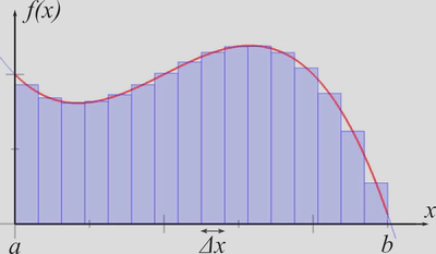
Let’s think of integration in a Riemann-like way: We have a function $f(x)$, and you take a particular interval $[a,b]$ of the variable $x$, with $a<b$, and split that interval into $N$ subintervals labelled by $i$, each having width $\Delta x = (b-a)/N$ and (say) central $x$ value of $x_i$, and then the integral $$\int_{[a,b]} f(x) \, \mathrm{d}x = \lim_{N \to \infty} \, \sum_{i=1}^N f(x_i) \, \Delta x .$$ This gives the (signed) area between the graph of $f(x)$ and the $x-$axis, between $a$ and $b$. The accompanying picture is the following (from Wikipedia):

The fundamental theorem of calculus is very intuitive from this picture if you think about adding/subtracting a rectangle at the right-hand/left-hand end of the interval $[a,b]$. It essentially says, in my notation, $$\begin{aligned} \frac{\mathrm{d}}{\mathrm{d}a}\int_{[a,b]} f(x) \, \mathrm{d}x &= -f(a) , \\ \frac{\mathrm{d}}{\mathrm{d}b}\int_{[a,b]} f(x) \, \mathrm{d}x &= f(b) . \end{aligned}$$ Often in fact only the second of those equations is called the fundamental theorem of calculus, and the first is considered something to be straightforwardly derived with what follows, but I like to think of the two statements arriving together, since they are clearly the same kind of idea, and could be derived in the same way.

Anyway, if you can find an antiderivative of $f$, i.e. a function $g(y)$ such that $g’(y) = f(y)$, then $$\int_{[a,b]} f(x) \, \mathrm{d}x = g(b) + \mathrm{constant} ,$$ because the right hand side is then a function of $b$ that has the same derivative with respect to $b$ as the function on the left hand side, so they can only differ by a constant. That’s because the difference of the two functions has zero derivative, and the only function with zero derivative is a constant (intuitive, but see the ‘Zero Velocity Theorem’ at math.stackexchange 91561). In our case the constant must equal $-g(a)$, because setting $b=a$ we must have $\int_{[a,a]} f(x) \, \mathrm{d}x = 0$.

Now, the way I like to think about things, $\Delta x$ and its infinitesimal limit $\mathrm{d} x$ are both always positive quantities; they are unsigned widths of intervals. There is no directionality in the integral - we’re not integrating ‘from left to right’ as opposed to ‘right to left’ of anything like that; in fact we could perform the sum over rectangles in any random order we like. Thus, things like (as people often write) $\int_a^b f(x) \, \mathrm{d}x = -\int_b^a f(x) \, \mathrm{d}x$ are in a sense notational shorthands in my way of thinking, and are arguably quite confusing or misleading. I’ve been especially confused before in the context of line integrals around a closed loop.

The ‘directionality’ only comes in when we start writing down antiderivatives, because they are directional; an antiderivative tells you how quickly a function changes as its argument increases. To illustrate a bit, let’s apply my way of thinking to integration by substitution.

We want to calculate $\int_{[a,b]} f(x) \, \mathrm{d}x$ where $a<b$ as before, and we have some other function $u(x)$ that is invertible in our interval (at least in principle) to get $x(u)$. Now, in my approach $$\int_{[a,b]} f(x) \, \mathrm{d}x = \int_{[c,d]} f(x(u)) \, \rule[-7pt]{0.4pt}{20pt} \frac{\mathrm{d}x}{\mathrm{d}u} \rule[-7pt]{0.5pt}{20pt} \, \mathrm{d}u ,$$ where $c<d$, because under the integral signs I take $\mathrm{d}x$ and $\mathrm{d}u$ to always be positive. So $$c, \, d = \begin{cases} u(a), \, u(b) & ~~\mathrm{if}~u(a) < u(b)\\ u(b), \, u(a) & ~~\mathrm{if}~u(a)>u(b) . \\ \end{cases}$$ Now lets assume that $\mathrm{sign}(\frac{\mathrm{d}x}{\mathrm{d}u})$ is constant over the interval in question. Thus $$\int_{[c,d]} f(x(u)) \, \rule[-7pt]{0.5pt}{20pt} \frac{\mathrm{d}x}{\mathrm{d}u} \rule[-7pt]{0.4pt}{20pt} \, \mathrm{d}u = \mathrm{sign}\left(\frac{\mathrm{d}x}{\mathrm{d}u} \right) \, \int_{[c,d]} f(x(u)) \, \frac{\mathrm{d}x}{\mathrm{d}u} \, \mathrm{d}u .$$ Now suppose we can actually evaluate the integral on the RHS using an antiderivative, by finding a function $g(u)$ such that $g’(u) = f(x(u)) \, \frac{\mathrm{d}x}{\mathrm{d}u}$. Then putting it all together we find $$\begin{aligned} \int_{[a,b]} f(x) \, \mathrm{d}x &= \mathrm{sign}\left(\frac{\mathrm{d}x}{\mathrm{d}u} \right) \, \left(g(d) - g(c) \right) \\ &= \begin{cases} \mathrm{sign}\left(\frac{\mathrm{d}x}{\mathrm{d}u} \right) \, \left(g(u(b)) - g(u(a)) \right) & ~~\mathrm{if}~u(a) < u(b)\\ \mathrm{sign}\left(\frac{\mathrm{d}x}{\mathrm{d}u} \right) \, \left(g(u(a)) - g(u(b)) \right) & ~~\mathrm{if}~u(a)>u(b)\\ \end{cases} \end{aligned}$$ But if $\mathrm{sign}\left(\frac{\mathrm{d}x}{\mathrm{d}u} \right) = 1$ then $u(a) < u(b)$, and if $\mathrm{sign}\left(\frac{\mathrm{d}x}{\mathrm{d}u} \right) = -1$ then $u(a) > u(b)$. Thus $$\boxed{ \int_{[a,b]} f(x) \, \mathrm{d}x = g(u(b)) - g(u(a)) \, .} \label{eqn:subst_result}\tag{1}$$ Now, what if $\mathrm{sign}(\frac{\mathrm{d}x}{\mathrm{d}u})$ is not constant over the integration interval? Well that’s fine; we just split the integration interval into sub-intervals, each with a constant $\mathrm{sign}(\frac{\mathrm{d}x}{\mathrm{d}u})$. Then eq. \ref{eqn:subst_result} holds for each sub-interval, and when we sum over the sub-intervals we find that eq. \ref{eqn:subst_result} in fact holds for the overall integral $\ddot\smile$.

The common way of writing all this is $$\begin{aligned} \int_a^b f(x) \, \mathrm{d}x &= \int_{u(a)}^{u(b)} f(x(u)) \, \frac{\mathrm{d}x}{\mathrm{d}u} \, \mathrm{d}u \\ &= \int_{u(a)}^{u(b)} g’(u) \, \mathrm{d}u \\ &= \big[ g(u) \big]_{u(a)}^{u(b)}\\ &= g(u(b)) - g(u(a)). \end{aligned}$$ I see this as a helpful shorthand and handle-turning method of getting the correct answer, without having to go through the hassle of my approach. That’s good, and it should be used! But I find my approach helpful to think about when I get confused about ‘integrating in a particular direction’. Basically by the time you get down to integrating a function of a variable over some interval, in an important sense that phrase doesn’t actually mean anything! Of course when doing a line integral the function may be e.g. a dot product with a tangent vector that points in a particular direction; that’s fine and represents a real directionality, but it’s a different thing to the fictional directionality that the common shorthand notation sometimes seems to imply.

My way of thinking also comes up when thinking about e.g. area integrals via a substitution, where writing down the new area element in my way of thinking involves the modulus of the determinant of the Jacobian, and the limits are arranged in ‘increasing size’ order as here; whereas again conventionally no modulus is involved, and the upstairs/downstairs integration limit notation is used without the size ordering.

P.S.
Here’s a cool little general result in closing (I saw it on Twitter, I think from Jim Al-Khalili but I’m not certain): $$\int_a^b f(a+b-x) \, \mathrm{d}x = \int_a^b f(x) \, \mathrm{d}x.$$ Amazingly, the proof of this cute thing is immediate upon just using the substitution $u = a+b-x$ and applying the usual ‘shorthand’ approach for integral limits and substitution that we’ve been discussing!

P.P.S.
Since we’re on the topic of integration, I recommend this cool recent paper ‘How to (Path-)Integrate by Differentiating’: https://arxiv.org/pdf/1507.04348.pdf
I do think they unhelpfully gloss their statement just under eq. 16 that $\partial_\epsilon^{-1}$ gives the antiderivative of the thing to its right. I think it essentially must follow from their statement just above eq. 5 that in general $f(\partial_\epsilon)$ should be interpreted as a function on the spectrum of $\partial_\epsilon$, which has eigenfunctions that are exponentials. So I guess the point is you write whatever is to the right of your $f(\partial_\epsilon)$ as a Fourier transform, and then use their eq. 5, and then you see that the result is that the thing to the right has been anti-differentiated (and I guess the constant chosen to be such that the Fourier transform of the anti-derivative, which we just wrote down, actually exists).