Why do distance functions satisfy an eikonal equation?

Every object has a scalar field associated with it called a distance function (DF), which equals the shortest distance from each point in space to the object. I think they’re quite beautiful things, and they’re extremely powerful tools in simulations (meshing, tracking interfaces) and graphics (ray marching, defining complex objects with simple expressions). Check out Inigo Quilez’s website and YouTube channel for lots of cool examples! To give a flavour, here’s a contour plot of one of Inigo’s:

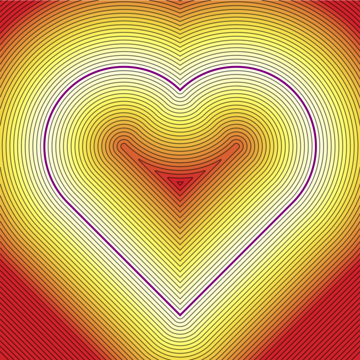
Fig. 1: Contour plot of distance $\phi$ from a heart (purple), coloured by $\phi$ with white = 0.

Let’s think in 2D (everything would generalise to higher dimensions straightforwardly). The DF $\phi$ of a curve $C$, satisfies the following special case of an eikonal equation: $$|\nabla \phi| = 1 \, , \label{eq:eikonal}\tag{1}$$ with the boundary condition $\phi=0$ on $C$. To me this equation always seemed plausible but not obviously correct, so I want to derive it. Hopefully you’ll at least agree with me going in that it’s fairly intuitive that a unique distance function does exist, because the question ‘how far am I from $C$?’ always has a single-valued answer, no matter where you’re standing.

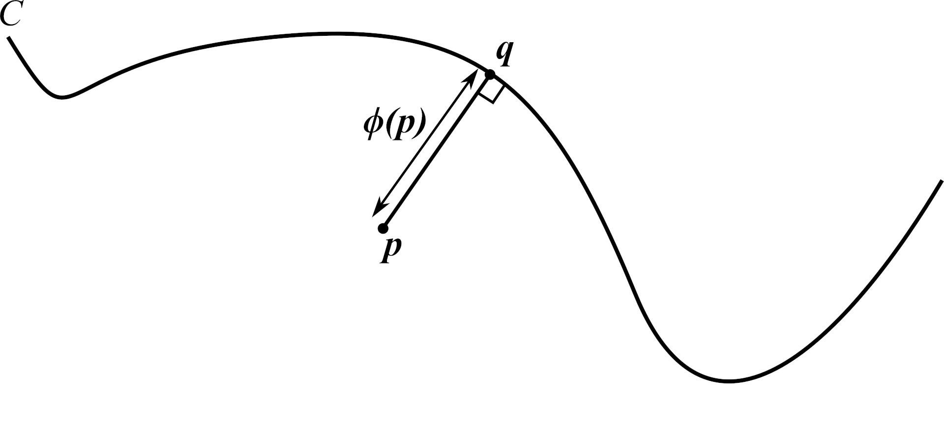
Fig. 2

The distance function $\phi(\mathbf{x})$ is a scalar field that equals the shortest distance from $\mathbf{x}$ to $C$. Let’s think about some particular point $\mathbf{x}=\mathbf{p}$. The shortest curve between two points is a straight line, so if the point on $S$ that’s closest to $\mathbf{p}$ is $\mathbf{q}$, the shortest distance from $\mathbf p$ to $S$ must be the length of the straight line from $\mathbf{p}$ to $\mathbf{q}$. Also, that line must meet $C$ at a right angle, because otherwise there would be a point $\mathbf q’$ on $C$ that’s closer to $\mathbf p$ than $\mathbf q$ is, by the triangle inequality (fig. 3a). Let’s call the unit tangent to that line $\hat{\mathbf t}$.

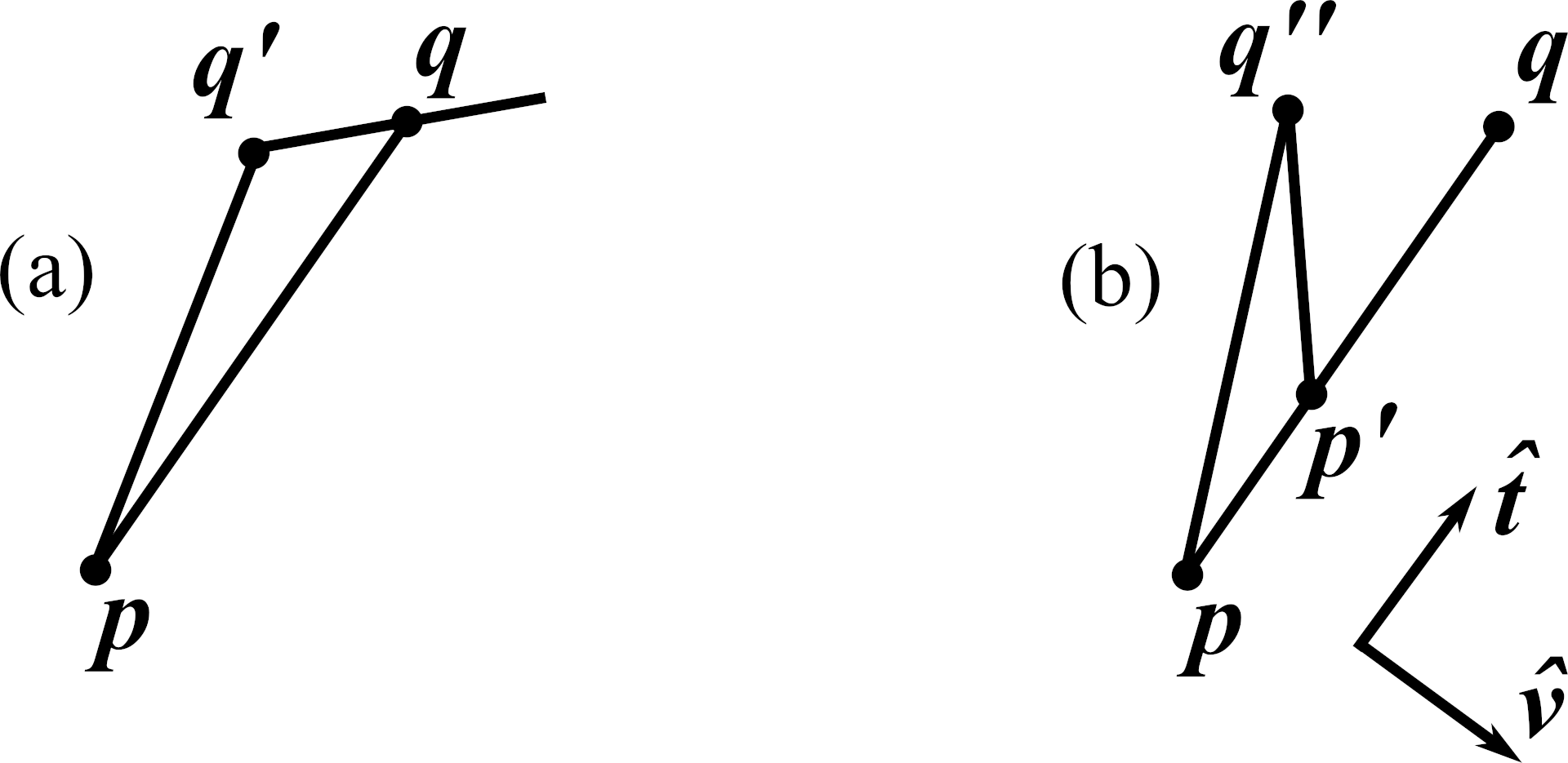
Fig. 3

Now, suppose we move from $\mathbf p$ towards $\mathbf q$ by some amount to arrive at $\mathbf p’ = \mathbf p + \lambda \hat{\mathbf{t}}$. Must the closest point on $C$ to $\mathbf p’$ also be $\mathbf q$? Yes! Otherwise there would be a point $\mathbf q’’$ on $C$ that closer to $\mathbf p$ than $\mathbf q$ is, by the triangle inequality (fig. 3b). Thus, the distance $\phi(\mathbf{p}’) = \phi(\mathbf{p}) - \lambda$, so letting $\lambda$ be infinitesimal we find the derivative of $\phi$ in the $\hat{\mathbf{t}}$ direction: $\nabla \phi \cdot \hat{\mathbf t} = -1$.

Let’s also find $\nabla \phi \cdot \hat{\mathbf v}$, the component in the perpendicular direction. To get going, here’s a sketch of what $C$ looks like locally near $\mathbf{q}$, where we’ve invented some $x$ and $y$ coordinates with the $y$-axis aligned along $\hat{\mathbf t}$.

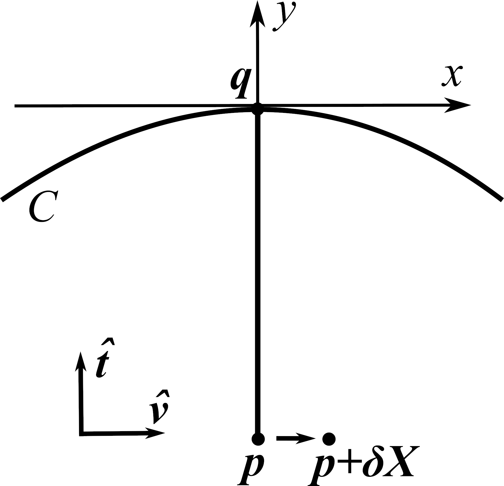
Fig. 4

Locally, $C$ is given to leading order by some quadratic $y = a x^2$ (parabola) with no linear term because, as discussed, $C$ must be perpendicular to $\hat{\mathbf t}$ at
$\mathbf{q}$. By Pythagoras, the squared distance $s$ from some point $(X,Y)$ to the point $(x,ax^2)$ on the parabola is $$s = (X-x)^2 + (Y-ax^2)^2 \, , \label{eq:sdef}\tag{2}$$ so the point on the parabola closest to the point $(X,Y)$ must have $x=x_c$ satisfying¹ $$\begin{aligned} \frac{\mathrm{d}s}{\mathrm{d}x}\rule[-7pt]{0.4pt}{20pt}\genfrac{}{}{0pt}{0}{}{\scriptstyle{x=x_c}} &= 0 \\ \implies X + 2 a Y x_c - 2 a^2 x_c^3 - x_c &= 0 \, . \end{aligned}$$ By construction, at $\mathbf{p}$ we have $X=0$ and the closest point is $\mathbf q = (0,0)$, and indeed $x_c=0$ solves the cubic in that case. Fixing $Y$ and considering $x_c$ as a function of $X$, we can differentiate the cubic implicitly to find $$\begin{aligned} &\frac{\mathrm{d}x_c}{\mathrm{d}X} = \frac{1}{1 + 6 a^2 x_c^2 - 2 a Y} \\ \implies &\frac{\mathrm{d}x_c}{\mathrm{d}X}\rule[-7pt]{0.4pt}{20pt}\genfrac{}{}{0pt}{0}{}{\scriptstyle{x_c=0}} = \frac{1}{1 - 2 a Y} \, . \end{aligned}$$ Thus, upon perturbing $X$ infinitesimally from 0 to $\delta X$ as shown in the sketch, we have $$\delta x_c = \frac{\delta X}{1 - 2 a Y}$$ to leading order. It is then easy to check from eqn (\ref{eq:sdef}) that $s(x_c)$ is only perturbed by $\mathcal{O}(\delta X^2)$ terms, as is the distance $\phi = \sqrt{s(x_c)}$. Thus, $\phi$ does not change to linear order if $\mathbf p$ is perturbed in the $\hat{\mathbf v}$ direction, i.e.
 $\nabla \phi \cdot \hat{\mathbf v} = 0$. If you want, it’s straightforward to go back and check that including higher-than-quadratic order terms in the local power series $y(x)$ does not change this moderately intuitive conclusion.

Phew! Now, $\hat{\mathbf t}$ and $\hat{\mathbf v}$ form a basis, so we have actually calculated $\nabla \phi$ in its entirety: $$\nabla \phi = - \hat{\mathbf{t}}. \label{eq:nabla_phi}\tag{3}$$ This means that if you’re at $\mathbf p$ and you want to decrease the distance to $C$ as quickly as possible you should walk straight towards $\mathbf{q}$, the closest point on the surface. Or, to flip it round, $\phi$ equals the shortest distance to $C$ and $-\nabla \phi$ is the direction of the straight line you should walk the distance $\phi$ along to reach $C$ as quickly as possible. Eqn (\ref{eq:nabla_phi}) immediately implies the eikonal
eqn (\ref{eq:eikonal}), since $\hat{\mathbf{t}}$ is unit length :)

It’s nice to check that the eikonal eqn agrees with the above observation that walking along $\nabla \phi$ should always mean walking in a straight line. To do so, we ask ‘how does $\nabla \phi$ change if we move by a tiny $\delta x$ along $\nabla \phi$’? We can calculate this change just using the grad of each component of $\nabla \phi$, finding $\delta \partial_i \phi = \delta x (\partial_j \phi) \partial_j (\partial_i \phi)$. This quantity equals 0, as you find quickly if you take $\partial_j$ of the eikonal eqn (\ref{eq:eikonal}) and use the symmetry of 2nd partial derivatives. So as we’d hope, every little step you take along $\nabla \phi$ brings you to a new point at which $\nabla \phi$ is the same as the point you were at before.

This straight lines thing should make one think of the method of characteristics, and indeed our eikonal equation (\ref{eq:eikonal}) has characteristics that are straight lines, as Zhao says just above eqn (2.9) in A fast sweeping method for eikonal equations. They are exactly the straight lines we’ve drawn and discussed already, which you walk along to get from $\mathbf p$ to $C$ as fast as possible. Eikonal equation characteristics are also called ‘rays’ because that’s exactly what rays in optics are. More general eikonal equations have a $\text{rhs} \neq 1$, which results in curved characteristics; see for example the nice paper Wavefronts and solutions of the eikonal equation by Nowack. That paper (p.56, top-right) makes clear that the characteristics $\mathbf{x}(\tau)$ have tangent vectors that equal $\nabla \phi$ for our case ($u=1, T = \phi$); in other words the straight characteristics are the integral curves of the vector field $\nabla \phi$.

We’ve explained why a DF satisfies the eikonal eqn (\ref{eq:eikonal}), but what about the inverse question: If I’ve found a function $\phi$ with $|\nabla \phi| = 1$ that has $\phi=0$ on $C$, can I be sure that that $\phi$ is in fact the DF of $C$? Only as long as you solved the eqn in a careful way! As fig. 1 demonstrates, there will generally be some kinks in the solution, because if you start solving the PDE locally from $C$ using the method of characteristics, eventually characteristics meet and the solution $\phi$ has kinks at these points. Technically you get something called a ‘viscosity solution’ — the name comes from the idea that you can regularize the problem by including a small viscosity term (2nd derivatives) in the equation, and then the kinky solution is the $\mathrm{viscosity} \to 0$ limit of the regularized solution. There are highly technical proofs of the uniqueness of viscosity solutions², but I don’t have much intuition for them, sadly. The fact that in general the solution necessarily has some kinks is a real pain, because there are infinitely many (Lipshitz-)continuous solutions that have kinks. To demonstrate, consider a 1D version of the problem: Solve $|\phi’|=1$ with BCs $\phi(0)=\phi(1)=0$. There are all sorts of kinky zig-zagging functions $\phi$ that satisfy this, but only the solution $\phi = 1- |x|$ is the distance function for the set $\{0,1\}$. Thankfully, if you solve by propagating ‘characteristics’ in from the two endpoints at equal speeds and stopping when they meet, this is exactly the solution you get — but the point is that just saying ‘we’re totally chill about kinks’ goes too far, because that would allow infinitely many solutions.

Really what we have to do is think about solving the PDE — and this is required for designing numerical methods too — in such a way that information propagates in particular fashion that ensures the resulting solution is the distance function solution. Hence the word ‘causality’ often comes up, and people use ‘upwind’ numerical schemes etc. So in some sense the bottom line is that there are not unique solutions to the eikonal eqn (\ref{eq:eikonal}), but there are ways to characterise the single solution that is the distance function, and to accordingly devise schemes that find that particular solution. Calder – Lecture notes on viscosity solutions (2018) seems to be very good on this stuff.